How LASSO Work

LASSO adds an L1 penalty to the regression loss function, encouraging sparse solutions by shrinking coefficients toward zero. Because the L1 penalty is not differentiable at zero, the optimization must be solved using subgradient, and it creates three piecewise equation, separately for the cases β_j > 0, β_j < 0, and β_j = 0. Solving the positive and negative cases yields valid solutions only when z_j > λ or z_j < −λ, respectively. When | z_j | ≤ λ, neither the positive nor negative solution is self-consistent, leaving β_j = 0 as the only valid optimum. Combining these three cases yields the soft-thresholding operator. As a result, coefficients with sufficiently large signal survive but are shrunk toward zero, while coefficients whose signal magnitude is smaller than the regularization threshold are set exactly to zero. This thresholding behavior is what gives LASSO its feature selection property.

Geometrically, the L1 constraint creates a diamond-shaped feasible region. The contours of the loss function often intersect this region at the corners, and those corners lie on the coordinate axes where one or more coefficients are zero. This provides an intuitive explanation for why LASSO tends to produce sparse solutions.

Definition

LASSO is a linear regression model with L1 regularization. Regularization intentionally introduces bias into coefficient estimates in exchange for lower variance, producing more stable and generalizable models. This results in more stable and generalizable models, even if the estimates are not as close to the true coefficients. It is a tug of war between getting the model as close to training data as possible, while also trying to keep the coefficient as small as possible.

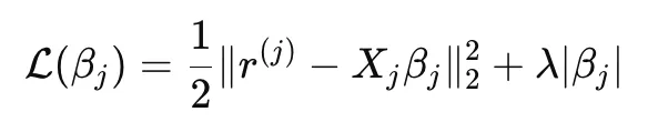
It minimizes:

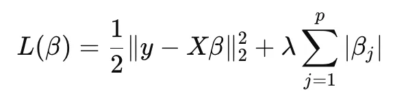
where:

• first term is the prediction error
• second term is the L1 penalty
• lambda controls the regularization strength

Note:

• We need to scale the variables because the coefficients directly affect the loss function, and coefficients are dependent on the size of the variables. If we don’t scale, large predictors with small coefficients will be penalized less.

• If relationship with x and y are non-linear, then LASSO may fail to capture

Constrained Form

The equivalent constrained optimization problem is:

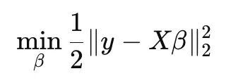
subject to:

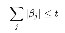
where t determines how large the coefficients are allowed to become.

Geometric: Why Coefficients to Zero

Terms

• Feasible Region - All coefficient values satisfying the constraint.
• Contour Line (Level Set) - All coefficient combinations producing the same loss value.

The unregularized squared-error loss forms elliptical contours around the OLS solution (as contour gets bigger, more the error).
The L1 constraint:

∣ β1 ∣ + ∣ β2 ∣ ≤ t

creates a diamond-shaped feasible region. The optimal solution is where the smallest loss contour first touches the feasible region. Because the diamond has sharp corners aligned with the axes, the intersection often occurs at a corner. At these corners, the β_j = 0.

For Ridge, the feasible region is a circle and since the boundary is smooth, intersections rarely occur exactly on an axis. Therefore Ridge shrinks coefficients but rarely sets them exactly to zero.

• L1 feasible region - diamond; these corners (axis-aligned) encourage zero coefficients.
• L2 feasible region - circle; smooth boundary → rarely hit exactly zero.

Algebraic: Why Coefficients to Zero

The L1 penalty is not differentiable at zero.

Its subgradient is:
![(1-1,1]](Attachments/B5AAAB29-F0E8-4830-993D-D6C4668B3A36.png)
Key intuition:

• For positive coefficients, the penalty contributes a constant slope of +1.
• For negative coefficients, the penalty contributes a constant slope of -1.
• Unlike Ridge, this pull toward zero does not weaken as the coefficient becomes small.
• Because the penalty is not differentiable at zero, we must consider three cases: β > 0, β < 0, and β = 0.
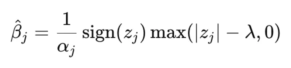
• Solving these three cases leads to the soft-thresholding operator.
• The soft-thresholding solution shows that coefficients with signal larger than the regularization threshold survive but are shrunk toward zero, while coefficients whose signal magnitude is smaller than the threshold are set exactly to zero.

The shrinkage force is proportional to the coefficient size, so it becomes weaker as the coefficient approaches zero. In contrast, the L1 penalty contributes a constant slope of ±1, which creates a thresholding effect that allows LASSO to produce exact zero coefficients and perform feature selection.

Soft-thresholindg/Coordinate Descent

Suppose we want to optimize only one coefficient βj while treating all other coefficients as fixed (coordinate descent). During CD, we fix everything except β_j to isolate the part of loss function involving β_j.

To rewrite the loss function in terms of β_j, we define partial residual r, which is the subtraction of y - y_pred without β_j:

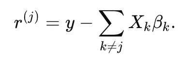
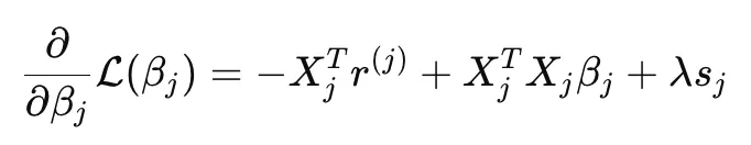
The loss function becomes:

When we take the gradient, we get in the form:

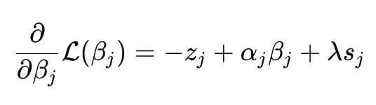
If we define the terms as:

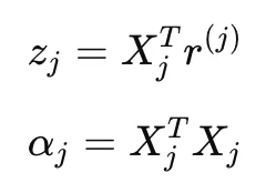
We can simplify the equation to:

• z_j: proportional to the correlation between predictor x_j and the remaining residual after subtracting the contribution of all other predictors from y
• α_j: x_j.T@x_j . If predictors are standardized, this is 1.
• s: subgradient

When we set the above equation to zero, there are three possible cases:

• β > 0 (subgradient is 1)
• β < 0 (subgradient is -1)
• β = 0 (subgradient is [-1, 1])

Then after solving the equation with the three different scenarios**:**

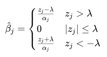
This can be conveniently be re-written as:

When the | z | is less than λ, the best solution is when β = 0. Note that z is the residual (y after subtracting y_hat that does not use x_j).

GLM Context

When adding L1 or Elastic Net penalties, the GLM objective becomes non-smooth due to the penality term λ| β_j |. This term has no Hessian and no derivative at zero. Therefore IRLS, Newton, BFGS, and CG cannot handle L1. Coordinate Descent solves this by updating one coefficient at a time.

This is the algorithm used by:

• statsmodels fit_regularized()
• H2O GLM
• glmnet in R

VIF vs LASSO

VIF measures linear dependency among predictors, not redundancy in predicting y. Therefore, variables can have low VIF yet still compete to explain the same residual variation in the target.

In this case, introducing variable X1 may substantially reduce the additional explanatory contribution of X2, causing LASSO to shrink X2 toward zero. However, if X1 is removed, X2 may once again explain meaningful residual variation and regain a nonzero coefficient.

If a variable x1 explains a large portion of the variance in y, then:

• Other variables that capture similar predictive structure — even if not strongly correlated with x1 — may be dropped
• This is because LASSO prefers sparse solutions and avoids retaining multiple predictors with overlapping explanatory contribution

Other Insights

• Uncorrelation doesn’t guarantee non-redundancy. They can be uncorrelated but still explain the same aspect of y, thus be redundant. Example: I made sure the variables are all under 3 for VIF. When I introduced variable X1, some variables like X3, X4 had 0 coefficients. But once I removed X1, the coefficients for X3 and X4 were no longer 0.
• Since LASSO uses the linear relationship of the variable and the residual for selecting variables, non-linear relationships will appear weak and will not be selected.